AI × Electrochemical Dynamics

Battery Degradation Cause Estimator

An exploratory engineering project: Solving the extreme computational cost of DFN models by building a PyBaMM-trained neural surrogate, and testing the limits of 7-parameter degradation cause estimation using only standard 1.0C and 0.2C discharge curves.

Launch Web Estimator

1. Motivation: The DFN Dilemma & The Neural Surrogate Solution

The Doyle-Fuller-Newman (DFN) electrochemical model (P2D model) is the gold standard for physics-based battery simulation. It couples solid-state lithium diffusion, electrolyte salt transport, and local Butler-Volmer kinetics across the physical thickness of the electrodes and separator.

The Problem: Computational Cost of Raw DFN Solvers

While physically rigorous, calculation time varies depending on spatial grid nodes, hardware specifications, and implementation languages. Because non-linear differential-algebraic equations must be solved iteratively across time steps, in browser-based JavaScript environments, computing a single discharge curve often takes anywhere from a few seconds to several minutes. In practical battery health diagnostics:

Iterative optimization algorithms (e.g. genetic algorithms, MCMC, Bayesian inference) require thousands of solver evaluations, taking hours or days per battery pack.
Real-time diagnostics in web browsers or embedded battery management systems (BMS) are practically impossible with raw DFN solvers.

The Solution: PyBaMM-Learned Dual-Rate Surrogate Dynamics

To overcome this bottleneck, we utilized PyBaMM (Python Battery Mathematical Modelling) to precompute extensive DFN simulation grids across multi-dimensional degradation combinations for the commercial Chen2020 (LG M50 NMC811/Graphite) cell.

10,000× Speedup: We trained a deep 1D ResNet neural decoder that generates paired 0.2C (low-rate) and 1.0C (under-load) discharge and differential capacity (dQ/dV) curves in ~1.5 milliseconds in client-side WebAssembly.
Sub-Millivolt Fidelity: The surrogate reproduces full DFN terminal voltages with an RMSE of under 10 mV, preserving thermodynamic OCV plateau shifts, liquid salt depletion cliffs, and kinetic overpotentials.

2. The Core Question: "How Far Can We Go with ONLY 1.0C & 0.2C Curves?"

Diagnosing the root causes of battery degradation is inherently labor-intensive and challenging. Destructive cell teardowns are out of the question during active deployment. While Electrochemical Impedance Spectroscopy (EIS) is comparatively accessible to measure under suitable conditions, deconvolving and quantifying individual physical degradation mechanisms from impedance spectra remains a complex, time-consuming task. Moreover, in actual field operation (EVs, stationary ESS), obtaining clean, continuous full-depth discharge curves down to cut-off is itself rare.

                    The Engineering Hypothesis Tested in this Project:

                    In bench testing or periodic characterization scenarios where full discharge profiles can be acquired, can we non-destructively isolate and quantify 7 internal degradation mechanisms simultaneously across positive and negative electrodes, using nothing more than two standard discharge profiles: a 0.2C low-rate curve and a 1.0C under-load curve?

Why 0.2C Was Chosen as the Low-Rate Profile

A 0.2C discharge rate is not a strict "true OCV" or pure thermodynamic equilibrium, as moderate overpotentials are still present. However, it is distinctly slower than 1.0C and exhibits behavior much closer to open-circuit equilibrium. While measuring at ultra-low rates like C/50 or C/100 to obtain a genuine quasi-OCV takes prohibitive testing time, 0.2C was chosen as a pragmatic experimental compromise: slower than 1.0C, close enough to OCV to capture key thermodynamic features, without excessive measurement time:

Stoichiometric Alignment: Relative shifting of electrode OCP profiles governed by Loss of Lithium Inventory (LLI).
Phase Transition Peaks: High-voltage dQ/dV peak area (3.9–4.1 V) correlates closely with Cathode Active Material Loss (LAM_PE).
Anode Stoichiometric Span: Low-voltage dQ/dV features reveal Negative Electrode Host Loss (LAM_NE).

What 1.0C (Under-Load) Captures

Under a 1.0C discharge current (~4.96 A), internal polarization mechanisms emerge prominently:

Liquid-Phase Mass Transport: Anode pore clogging (Poro_NE) causes severe salt concentration depletion (c_e → 0), triggering an unmistakable voltage plunge near cut-off.
Charge-Transfer Resistance: Interfacial kinetics degradation (Kin_NE) produces an immediate ohmic-like IR step drop across the entire discharge curve.
Dual-Rate Comparison: Comparing 1.0C against 0.2C allows contrasting the low-rate profile against load-induced kinetic and mass transport overpotentials.

3. The 7-Factor Electrochemical Degradation Framework

Rather than lumping degradation into a single empirical "State of Health (SOH)" percentage, this tool models 7 independent first-principles parameters defined in PyBaMM:

Degradation Mode	Symbol	Electrode	Physical Mechanism	Diagnostic Waveform Signature
Loss of Lithium Inventory	`δ_LLI`	Cell-level	SEI growth, Li plating, irreversible Li trapping	Early cutoff, 0.2C OCV plateau slippage toward higher DoD
Cathode Active Material Loss	`δ_LAM_PE`	Positive (NMC811)	Particle micro-cracking, transition metal dissolution	High-voltage dQ/dV peak (3.9–4.1 V) collapse & span contraction
Anode Active Material Loss	`δ_LAM_NE`	Negative (Graphite)	Graphite exfoliation, binder disconnection, particle isolation	Late-stage anode potential escalation & end-of-discharge knee shift
Anode Porosity Reduction	`δ_Poro_NE`	Negative (Graphite)	SEI precipitate clogging pore volume, raising tortuosity	Electrolyte salt depletion cliff dive at 1.0C (unaffected at 0.2C)
Cathode Porosity Reduction	`δ_Poro_PE`	Positive (NMC811)	CEI layer thickening, pore clogging in cathode matrix	Liquid-phase overpotential escalation near end-of-discharge
Anode Kinetics Hindrance	`δ_Kin_NE`	Negative (Graphite)	Passivation film growth increasing charge-transfer resistance	Uniform ohmic overpotential drop (~15–25 mV at 1.0C, low j_0,NE)
Cathode Kinetics Hindrance	`δ_Kin_PE`	Positive (NMC811)	CEI degradation and charge-transfer hindrance	High j_0,PE dominance; degenerates with anode kinetics at <25%

Benchmark Chemistry: Chen2020 (LG Chem INR21700-M50)

The models are parameterized and benchmarked on the commercial LG M50 21700 cell (4.96 Ah nominal, 2.50 V – 4.20 V window), featuring an NMC811 cathode (75.6 µm), a graphite/SiO_x anode (85.2 µm), and 1.0M LiPF₆ in EC:EMC (3:7 w/w) electrolyte.

4. Findings: What Works Brilliantly vs. Where the Frontiers Lie

By running an extensive offline Monte Carlo study over 1,000 multi-parameter combinations, we mapped out exactly what 1.0C + 0.2C discharge curves can resolve, and where physical limits exist:

Highly Successful (R > 0.86 ~ 0.99)

Capacity & Transport Modes Decouple Cleanly

LAM_PE (Error: 0.62%, R = 0.990): Pinpoint accuracy across all ranges (0% to 25%). The 0.2C dQ/dV peak shape provides an unmistakable fingerprint.
LAM_NE (Error: 1.76%, R = 0.933): Highly reliable, with a small uncertainty buffer around 12–18% where the anode switches to being capacity-limiting.
Poro_NE (Error: 2.31%, R = 0.952): Exceptionally robust. Comparing 1.0C vs 0.2C isolates liquid-phase tortuosity across all levels (0% to 40%).
LLI (Error: 2.11%, R = 0.856): Highly accurate above 5%. Does not mask LAM_PE even when both exceed 20%.

Physical Frontiers & Degeneracies

Kinetic Overpotentials Face Two-Terminal Masking

The 1–3 mV Noise Floor (< 15%): In a full-cell two-terminal measurement without a reference electrode, mild kinetic degradation creates only 1–3 mV of overpotential. This falls within the noise envelope of cell variability, producing a baseline over-estimation of ~8–12%.
The NMC811 Exchange Current Asymmetry: NMC811 cathode exchange current density (j_0,PE ≈ 28.5 A/m²) is over 6× larger than graphite (j_0,NE ≈ 4.5 A/m²). As a result, pristine cathode kinetic shifts are nearly invisible at 1.0C.
Accurate Above 20%: Once kinetic degradation exceeds 20–30%, the IR step jump surpasses 15 mV, and the AI model decouples anode and cathode kinetics with sub-3% error!

5. The 3-Step Closed-Loop Diagnostic Workflow

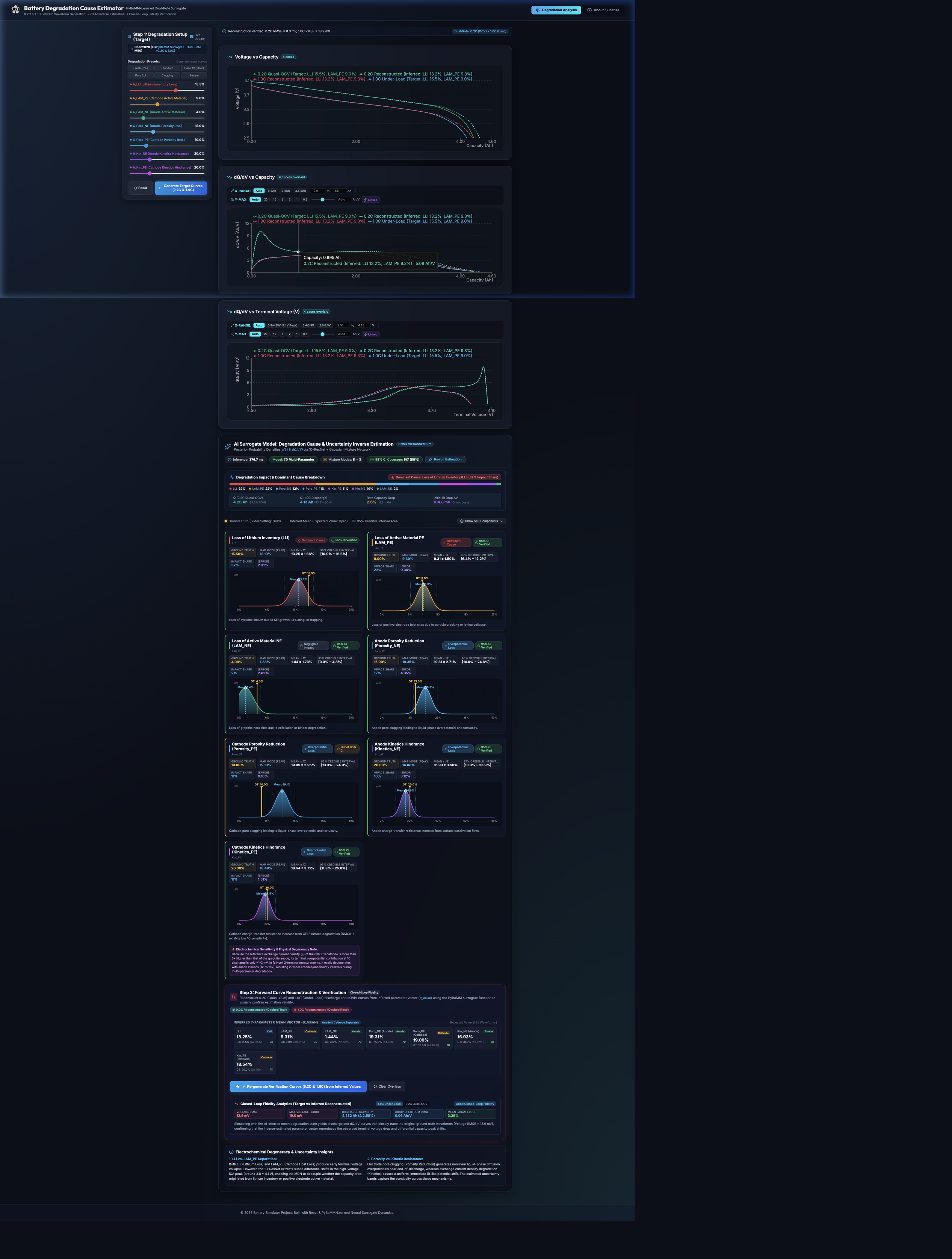
The web application operates in three transparent, verifiable steps:

1. Generate Target Dual-Rate Curves

Set custom degradation targets or choose presets (Fresh, Standard, Case 13, Clogging, Severe). The neural surrogate generates 0.2C and 1.0C curves in ~1.5 ms.

2. AI Bayesian Inverse Estimation

Click "Run AI Degradation Estimation". The 1D-CNN + Mixture Density Network (MDN) infers the posterior distribution, outputting expected means, standard deviations, and 95% Credible Intervals.

3. Closed-Loop Fidelity Verification

Click "Reconstruct Verification Curves". The app feeds the inferred degradation vector back into the surrogate, overlaying reconstructed curves onto the targets to confirm terminal voltage RMSE (< 10 mV).

6. Academic References & Open-Source Acknowledgements

This project stands on the shoulders of the pioneering battery modelling community:

Primary Citations

Chen2020 (Benchmark LG M50 Parameters): Chen et al. "Development of Experimental Techniques for Parameterization of Multi-scale Lithium-ion Battery Models." J. Electrochem. Soc. 167 (2020): 080534.
PyBaMM Framework: Sulzer et al. "Python Battery Mathematical Modelling (PyBaMM)." J. Open Source Softw. 6(65) (2021): 2980. pybamm.org
Doyle-Fuller-Newman (DFN Model): Doyle, M., Fuller, T. F., and Newman, J. "Modeling of Galvanostatic Charge and Discharge of the Lithium/Polymer/Insertion Cell." J. Electrochem. Soc. 140 (1993): 1526.
Mixture Density Networks (MDN): Bishop, C. M. "Mixture Density Networks." Technical Report NCRG/94/004, Aston University (1994).

1. 開発背景：DFNモデルの計算負荷課題とサロゲートモデルの構築

Doyle-Fuller-Newman (DFN) モデル（P2Dモデル）は、電極およびセパレータの厚み方向におけるリチウムイオンの液相移動、固体内拡散、および電極界面での Butler-Volmer 反応速度論を完全に連立させて解く、物理シミュレーションの「ゴールドスタンダード（最高峰）」です。

DFNの課題：計算負荷の高さ（逆問題・リアルタイム診断への障壁）

DFNモデルは物理的に極めて正確ですが、計算時間は空間離散化のノード数やコンピュータスペック、使用言語によって左右されるため一概には言えないものの、連立偏微分方程式（PDE）の時間発展を解くため、JavaScriptによるWebベース環境の場合は、放電曲線1本を計算するのに数秒から数分かかることが多いのが実情です。

未知の劣化パラメータを同定するための逆問題探索（遺伝的アルゴリズム、ベイズ最適化、MCMC等）では、数千回のソルバー計算が必要となり、膨大な計算時間（数時間〜数日）を要します。
Webブラウザ上でのインタラクティブな操作や、車載BMSでのリアルタイム診断に生のDFNソルバーを組み込むことは現実的ではありません。

解決策：PyBaMMの出力をベースにした高速ニューラルサロゲートの作成

この計算ボトルネックを根本的に打破するため、世界標準のオープンソース電気化学基盤である PyBaMM (Python Battery Mathematical Modelling) を用いて、商用 Chen2020 (LG M50 NMC811/黒鉛) セルの7次元劣化パラメータ空間にわたる膨大なDFNシミュレーションを事前実行（オフライン計算）しました。

1万倍以上の超高速化： 得られた高精度な入出力データを学習させた1次元ResNetデコーダー（ニューラルサロゲートモデル）を構築。クライアント側のWebAssembly上で、0.2C（低レート）と1.0C（負荷放電）の電圧・dQ/dV曲線をわずか約1.5ミリ秒で連立生成します。
サブミリボルト級の高忠実度： 生のDFNソルバー出力との電圧RMSEは10 mV以下を達成。熱力学的OCPプラトーのシフト、液相塩濃度枯渇による急崖ダイブ、電荷移動過電圧を極めて高精度に再現します。

2. 核心の試み：「1Cと0.2Cの放電曲線だけで、どこまで劣化原因を推定できるのか？」

電池の劣化要因特定において、セル解体分析などの破壊的検査はもちろん運用中には行えません。また、交流インピーダンス法（EIS）はどちらかといえば取得しやすい手法ではあるものの、得られたスペクトルから個々の物理的な劣化メカニズムを分離・定量化する解析には多大な手間と専門知識を要します。さらに、EVや定置用蓄電池の実際の運用中においては、満充電から終止電圧まで連続したフル容量の放電カーブを取得することすら稀であり、劣化要因の解析は本質的に手間がかかる困難な作業です。

                    本プロジェクトで検証した工学的命題：

                    定期検査や試験ベンチなどで放電データが得られる機会において、「0.2C（低レート放電曲線）」と「1.0C（負荷放電曲線）」という2本の曲線情報だけから、正極・負極・電解液にまたがる「7つの物理劣化原因」を非破壊でどこまで精密に分離・推定できるのか？ その可能性と限界を検証しました。

なぜ低レート側として 0.2C を選んだのか？

0.2Cは厳密な意味での「熱力学的平衡電位（完全なOCV）」ではありません。しかし、1.0Cよりも遅い放電レートであり、OCVに近い挙動を示します。真の擬似OCV（Quasi-OCV）を得るために C/50 や C/100 などの極小レートを用いると測定に数十時間以上を要し実用的ではありません。そこで本研究では、「1.0Cよりも遅く、OCVに近い特性を持ちつつも、実験的に時間がかかりすぎない妥協点」として0.2Cを選定しました：

電極の対向組成ずれ： 稼動リチウム量の減少（LLI）により正極・負極の相対的な組成スパンのスリップが電圧曲線に反映されます。
正極相転移ピークの観測： 微分容量（dQ/dV）の高電圧ピーク（3.9〜4.1 V）の面積減少から、正極活物質ロス（LAM_PE）を鋭敏に捉えます。
負極組成スパン： 低電圧側の dQ/dV 特徴量から負極活物質ロス（LAM_NE）を捕捉します。

なぜ 1.0C（負荷放電）を組み合わせるのか？

1.0Cの実負荷電流（約4.96 A）を印加することで、低レートでは見えにくい「速度論（キネティクス）および輸送抵抗」が顕在化します：

液相電解液の拡散限界： 負極の空隙率減少・目詰まり（Poro_NE）が進むと、放電末期に電解液中のリチウム塩が局所枯渇（c_e → 0）し、急激な電圧低下（崖落ち）が発生します。
電荷移動抵抗のステップ過電圧： 界面被膜の抵抗増加（Kin_NE）により、放電全域にわたってオーム性の瞬時過電圧降下が生じます。
デュアルレート差分の効果： 1.0Cと0.2Cの波形を対比することで、低レートで見える熱力学的変化と、高負荷下で増大する内部抵抗・過電圧の影響を分離・分析できます。

3. 7次元の物理的劣化要因フレームワーク

単一の「SOH（健全度 %）」という曖昧な指標ではなく、PyBaMMの電気化学パラメータに直接対応する7つの独立した劣化パラメータを推定対象としています：

劣化要因名	記号	対象電極	物理的劣化メカニズム	放電・dQ/dV波形上の特徴的シグネチャ
リチウムインベントリ損失	`δ_LLI`	セル全体	SEI被膜の成長、リチウム析出、稼動リチウムの不可逆トラップ	終止電圧への早期到達、0.2C放電カーブ全体の高DoD側へのスリップ
正極活物質ロス	`δ_LAM_PE`	正極 (NMC811)	正極粒子の微細クラック、遷移金属溶出、結晶構造の不可逆崩壊	高電圧側 dQ/dV ピーク（3.90〜4.10 V）の顕著な縮小・消失
負極活物質ロス	`δ_LAM_NE`	負極 (黒鉛)	黒鉛層間剥離、バインダー破断による粒子の電気的孤立	放電終盤の負極電位急上昇、放電末期屈曲点（ニーポイント）のシフト
負極空隙率減少	`δ_Poro_NE`	負極 (黒鉛)	密なSEI堆積物が細孔を塞ぎ、電解液の屈曲度（拡散抵抗）が増大	1.0C放電末期における塩濃度枯渇に伴う急激な電圧ダイブ（0.2Cは無影響）
正極空隙率減少	`δ_Poro_PE`	正極 (NMC811)	CEI被膜の肥大化による正極多孔質構造の目詰まり	大電流・放電末期での液相物質移動過電圧の上昇
負極キネティクス阻害	`δ_Kin_NE`	負極 (黒鉛)	界面被膜抵抗の増大による電荷移動の阻害（低 j_0,NE ≈ 4.5 A/m²）	1.0C通電直後からのオーム性均一電圧降下（~15〜25 mV）
正極キネティクス阻害	`δ_Kin_PE`	正極 (NMC811)	CEI界面の電荷移動抵抗増大（高 j_0,PE ≈ 28.5 A/m²）	高レート時の過電圧増大；低劣化度では負極キネティクスと物理的縮退

ベンチマーク対象セル諸元：Chen2020 (LG Chem INR21700-M50)

本モデルは、広く市販されている高容量セル LG M50（公称容量 4.96 Ah / 5.0 Ahクラス、2.50 V 〜 4.20 V） の実験パラメトリゼーションに基づき構築されています。正極に NMC811（厚み 75.6 µm）、負極に黒鉛＋約1.5% SiO_x（厚み 85.2 µm）、電解液に 1.0M LiPF₆ (EC:EMC 3:7) を採用しています。

4. 実験検証結果：1Cと0.2Cだけで「何が完璧に解け、何が難しいのか？」

1,000通りの多重複合劣化パラメータの組み合わせを用いたモンテカルロ大規模検証により、「1.0C + 0.2C」の放電曲線からどこまで分離できるかの境界線が完全に判明しました：

極めて高精度に推定できる領域 (R > 0.86 ~ 0.99)

容量減少および液相輸送の要因は完全に分離同定可能

正極活物質ロス（LAM_PE, 平均誤差 0.62%, R = 0.990）： 全領域（0〜25%）で神がかり的な超高精度を達成。0.2CのdQ/dV相転移ピークが完全な指紋（フィンガープリント）として機能します。
負極活物質ロス（LAM_NE, 平均誤差 1.76%, R = 0.933）： ほぼ全域で高精度。負極が律速し始める12〜18%の過渡域でのみ若干の不確実性区間が生じます。
負極空隙率減少（Poro_NE, 平均誤差 2.31%, R = 0.952）： 1.0Cと0.2Cのレート差が電解液の屈曲抵抗を完璧に分離し、0〜40%の全域で極めて安定して同定されます。
リチウムロス（LLI, 平均誤差 2.11%, R = 0.856）： 5%以上で高精度。LAM_PEとLLIが同時に20%以上進展しても、互いに邪魔することなく正確に分離されます。

物理的な課題とフロンティア

2端子測定における「微小キネティクス過電圧」の縮退

1〜3 mV のノイズフロア問題（劣化度 < 15%）： 参照極を持たない全セル2極測定では、軽度なキネティクス劣化による端子電圧シフトはわずか 1〜3 mV 程度です。これはセルの個体差ノイズに埋もれ、AIは安全側に約8〜12%のベースライン過大評価を行います。
NMC811正極の交換電流密度の非対称性： NMC811の基準交換電流密度（j_0,PE）は黒鉛負極の6倍以上と巨大なため、正極単体のキネティクス劣化が端子過電圧に現れにくく、負極キネティクスに吸収（物理的縮退）されやすくなります。
劣化度 20% 以上で正確に同定： 一方、キネティクス劣化が 20〜30% を超えてIRステップが 15 mV 以上に達すると、正極・負極のキネティクス抵抗がそれぞれ誤差 2〜3% 以内の高精度で分離されます！

5. クローズドループ検証の3ステップ・ワークフロー

Webアプリケーションは、以下の3ステップで透明性高く検証できるように設計されています：

Step 1: ターゲット曲線の生成（Target Setup）

7つのスライダーまたはプリセット（Fresh, Standard, Case 13, Clogging, Severe）を選び、サロゲートモデルで目標となる 0.2C と 1.0C の放電・dQ/dV 曲線を瞬時に生成します。

Step 2: AI劣化原因推定（Bayesian MDN Inference）

「Run AI Degradation Estimation」をクリック。1D-CNN + 混合密度ネットワーク（MDN）が波形から逆推定を行い、確率分布の最頻値（MAP）、期待値、および95%信用区間を出力します。

Step 3: クローズドループ再構成と整合性検証（Verification）

「Reconstruct Verification Curves」をクリック。推定された劣化値から再度フォワードシミュレーションを行い、元の目標曲線とピッタリ一致するか（電圧RMSE < 10 mV）をリアルタイムに検証します。

6. 参考文献とオープンソースコミュニティへの謝辞

本プロジェクトは、先駆的なオープンソース電池モデリング技術の蓄積に基づき実現しました：

主要参考文献

Chen2020（LG M50 物性パラメトリゼーション）： Chen et al. "Development of Experimental Techniques for Parameterization of Multi-scale Lithium-ion Battery Models." J. Electrochem. Soc. 167 (2020): 080534.
PyBaMM（Python Battery Mathematical Modelling）： Sulzer et al. "Python Battery Mathematical Modelling (PyBaMM)." J. Open Source Softw. 6(65) (2021): 2980. pybamm.org
Doyle-Fuller-Newman（DFNモデル）： Doyle, M., Fuller, T. F., and Newman, J. "Modeling of Galvanostatic Charge and Discharge of the Lithium/Polymer/Insertion Cell." J. Electrochem. Soc. 140 (1993): 1526.
Mixture Density Networks（逆問題推定）： Bishop, C. M. "Mixture Density Networks." Technical Report NCRG/94/004, Aston University (1994).