A comprehensive web platform integrating Single Particle Model with Electrolyte (SPMe), physical degradation kinetics (LLI, LAM, Contact Resistance), and Arrhenius thermal acceleration to calibrate and predict long-term battery degradation under real-world temperature distributions.
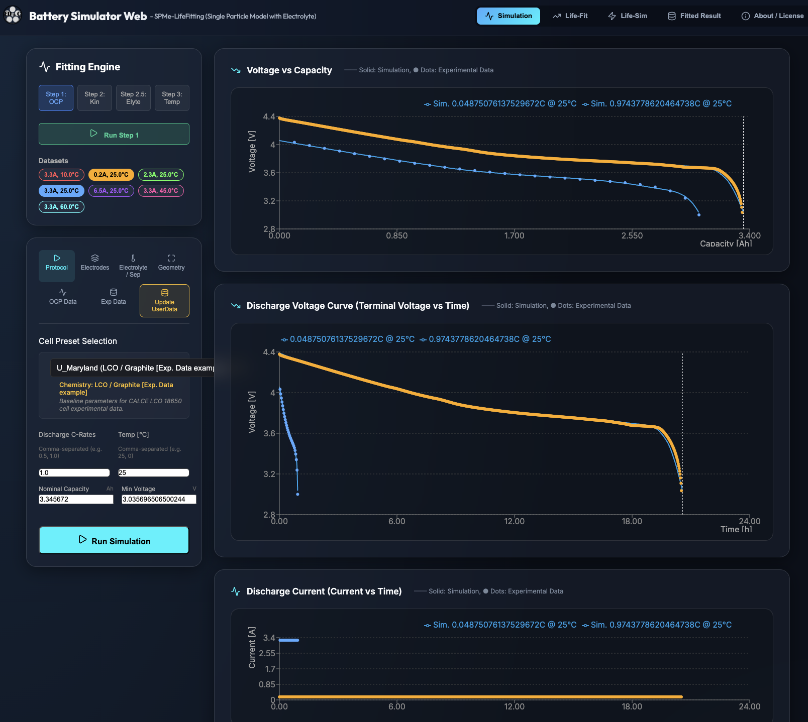
Battery Simulator Web — SPMe-LifeFitting seamlessly couples macro-scale electrochemical dynamics with degradation mechanics. It comes pre-loaded with curated open-access datasets for immediate calibration and lifetime prediction.
The application leverages open-access accelerated cycle life testing datasets provided by the University of Maryland Center for Advanced Life Cycle Engineering (UMD CALCE). The benchmark battery is a commercial pouch cell featuring LiCoO2 (LCO) Cathode, Graphite Anode, and 3360 mAh Nominal Capacity, tested across multiple ambient thermal conditions (25°C, 45°C, and 60°C).
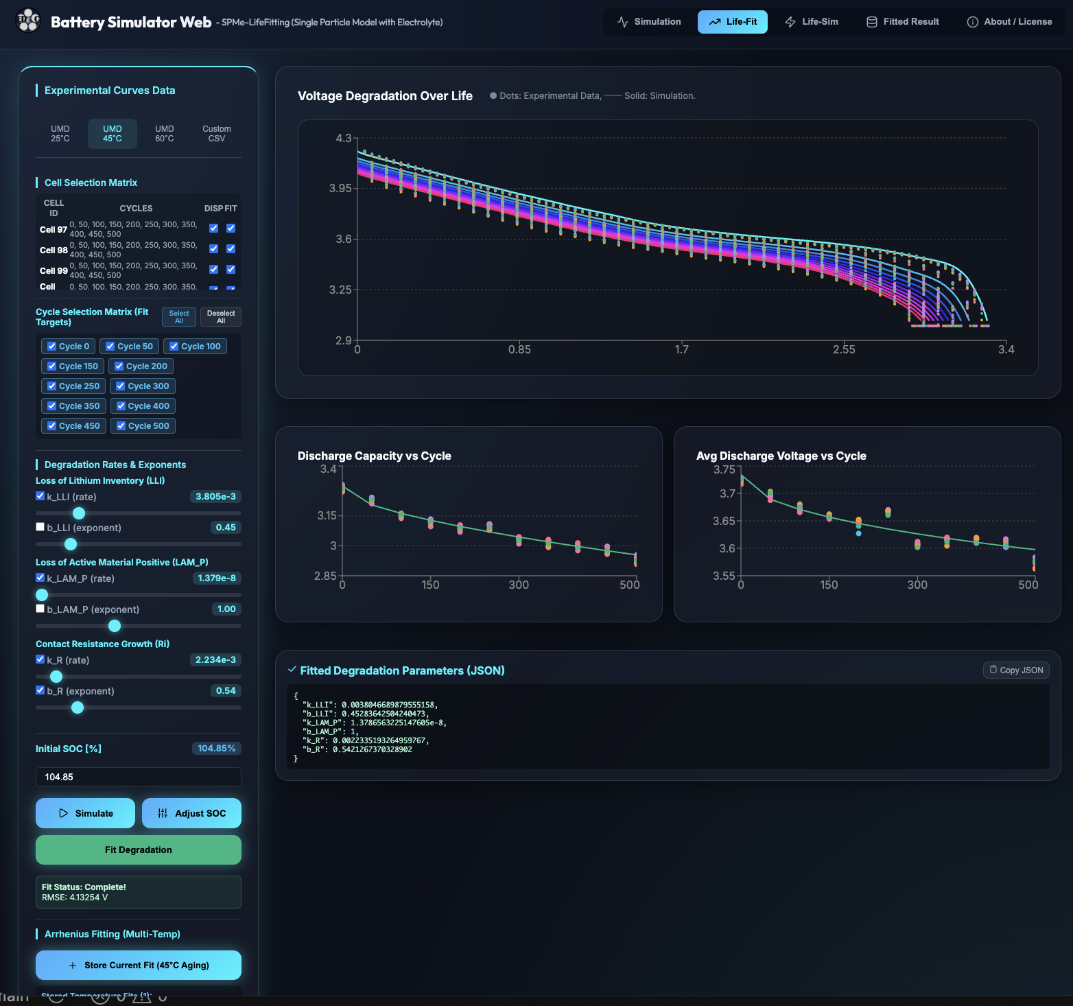
The "Life-Fit" module calibrates physical degradation parameters against experimental discharge curves cycled under three distinct ambient temperatures (25°C, 45°C, and 60°C).
Key Environmental Premise: While cycle aging tests are executed under different ambient temperatures (25°C, 45°C, 60°C), post-cycling discharge characterizations and capacity evaluations are always conducted under a unified standard room temperature (25°C).
Why is Adjust SOC necessary?
Baseline physical parameters are inherited from the fresh cell calibration. However, the
charging protocols and cutoff current conditions used during continuous cycle aging differ
from those applied during post-aging capacity evaluation tests. Consequently,
fine-tuning the initial State of Charge (Initial SOC) right before discharge is required to
align the discharge voltage knee.
The degradation model tracks three major physical failure modes following power-law kinetics:
L_LLI(N) = k_LLI · N^(b_LLI)L_LAM_P(N) = k_LAM_P · N^(b_LAM_P)ΔR(N) = k_R · N^(b_R)b_LLI, b_LAM_P, b_R) represent temperature-independent physical constants.k_LLI, k_LAM_P, k_R) at 45°C and
60°C.
Fit Degradation to optimize k, then click Simulate to
render capacity fade, voltage drop, and experimental overlay. Repeat until satisfactory
convergence is achieved.
Store Current Fit to save the fit into
Arrhenius memory, then proceed to the next temperature.
Fit Arrhenius Model. The engine extracts activation energies
(Ea) and pre-exponential factors (kref) via log-linear
least squares regression.
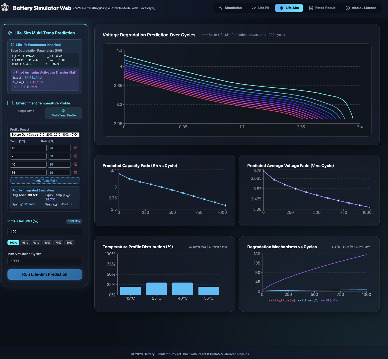
Real-world battery applications (EVs, BESS, consumer electronics) experience time-varying thermal distributions rather than single constant temperatures.
The "Life-Sim" panel computes Effective Degradation Rate Constants taking into account Arrhenius non-linearities across user-defined thermal frequency distributions (e.g., 25°C 50%, 45°C 30%, 60°C 20%), simulating long-term capacity fade, average voltage decay, and discharge curve evolution over thousands of cycles.
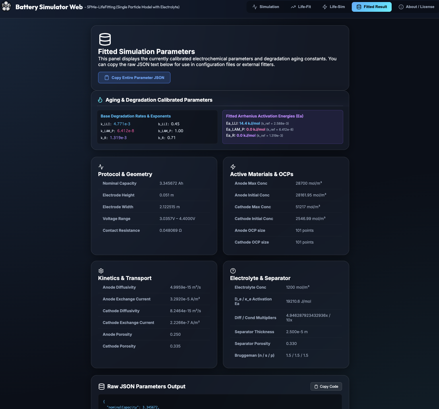
The "Fitted Result" tab provides a comprehensive single-page summary of all calibrated electrochemical parameters, physical geometry, and degradation aging constants (k, b, Ea). One-click JSON export is provided for seamless integration into external modeling pipelines (such as PyBaMM or Python scripts).
Battery Simulator Web — SPMe-LifeFitting は、公開されている学術実測データをプリセットとして活用し、電池の初期物理特性のフィッティングから、サイクル進行に伴う劣化同定・アレニウス温度依存性の算出・将来の寿命予測までを直感的に行える物理モデルプラットフォームです。
本アプリでは、米国メリーランド大学 Center for Advanced Life Cycle Engineering (UMD CALCE) から公開されている市販リチウムイオンパウチセル(LiCoO2 / LCO 正極, グラファイト負極, 定格 3360 mAh)の多温度(25°C, 45°C, 60°C)サイクル加速寿命試験データを標準プリセットとして標準搭載しています。
「Life-Fit」タブでは、3種類の異なるエージング環境温度(25°C, 45°C, 60°C)でサイクル進行させた放電曲線データに対し、物理的劣化パラメータの同定を行います。
重要前提条件: サイクル試行時のエージング環境温度(25°C, 45°C, 60°C)はそれぞれ異なりますが、サイクル経過後の容量・放電性能評価はすべて同一の標準温度環境(25°C)で統一測定されています。
なぜ Adjust SOC の調整が必要なのか?
初期性能同定(Simulation
タブ)のパラメータを基本の物理パラメータとして採用していますが、「サイクル試験時の充電プロトコル」と「サイクル経過後の性能評価測定における充電条件(カットオフ電流・満充電規定)」が異なるため、サイクル後の放電曲線を正確にフィッティングするには放電開始直前の初期
SOC (Initial SOC) を微調整する必要があります。
モデルでは電池の主要な 3 大物理劣化機構を以下の冪乗法則(Power-law)に従って同定します:
L_LLI(N) = k_LLI · N^(b_LLI)
L_LAM_P(N) = k_LAM_P · N^(b_LAM_P)
ΔR(N) = k_R · N^(b_R)b_LLI, b_LAM_P, b_R)は温度に依存しない物理定数(共通値)として扱います。k_LLI, k_LAM_P, k_R)のみを最適化します。
Fit Degradation ボタンを押して速度定数 k を最適化します。続けて Simulate
ボタンを押すことで、容量劣化、平均放電電圧の低下、放電曲線の変化が描画されます。満足のいくフィッティングが得られるまでこれを繰り返して最適値を探します。
Store Current Fit
ボタンを押してアレニウスフィッティング用にデータを一時格納し、次の温度条件の同定へ移ります。
Fit Arrhenius Model
を実行し、活性化エネルギー(Ea)と基準速度定数(kref)を算出します。
実際の電池アプリケーション(電気自動車 EV、家庭用・産業用蓄電池、スマートフォン等)では、環境温度は一定ではなく地域や季節により変動し時間分布(頻度割合)を持ちます。
「Life-Sim」タブでは、設定入力された環境温度プロファイル(例: 25°C 50%、45°C 30%、60°C 20%)の頻度を想定し、アレニウス効果を加味した**等価実効劣化速度定数 (Effective Degradation Rates)** を算出し、サイクル劣化後の放電カーブやその変化を高精度にシミュレーションします。
@misc{kusachi2025lifefit,
  author = {Yuki Kusachi},
  title = {Battery Simulator Web - SPMe-LifeFitting (Degradation Kinetics \& Lifetime)},
  year = {2025},
  url = {https://www.edandc.com/BattSimWeb-LifeFit/},
  note = {YK Energy Device \& Consulting}
}