
EIS-DRT-Excel-Analyzer
~ Empowering Engineers with Advanced DRT Analysis Beyond Corporate IT Security Constraints ~
1. Introduction: The Mission Behind This Project
Distribution of Relaxation Times (DRT) analysis is a powerful tool for deconvolving physical phenomena from Electrochemical Impedance Spectroscopy (EIS) data. While cloud-based analysis services exist, many engineers handling sensitive data face significant barriers due to corporate IT security policies that prohibit uploading data to external servers.
This project aims to "complete professional-grade DRT analysis entirely within local Excel environments." Provided as VBA code, this tool allows you to bypass strict software installation restrictions and conduct advanced analysis securely on your desktop without ever sending your confidential data outside your organization.
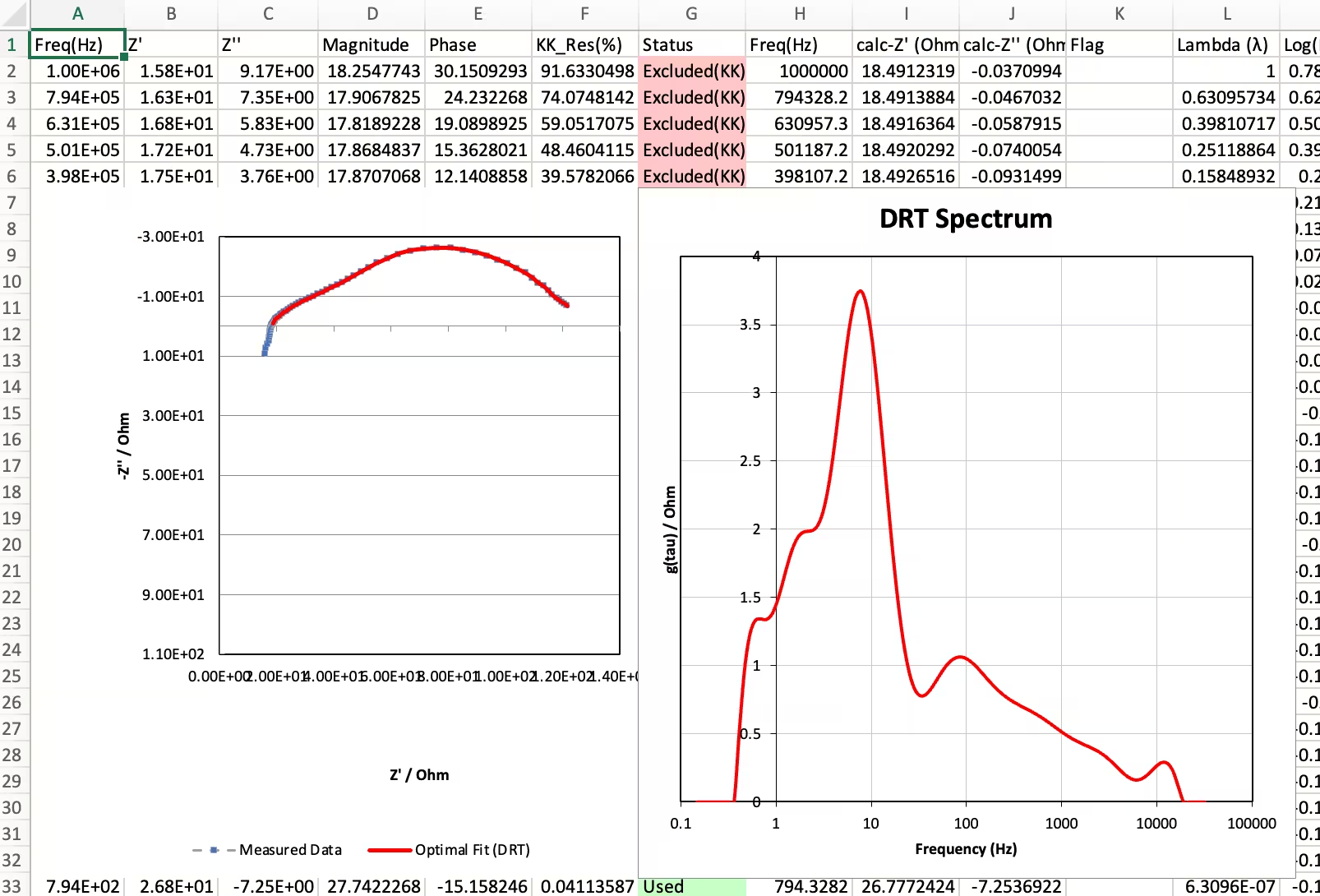
2. Usage
GitHub Repository: @ykusachi/Excel_DRT
You can copy the VBA source code or download template files from the link above.
Module Configuration
DRT_core.bas: The core DRT algorithm. Derives the distribution function from a single set of impedance data.Z_summary.bas: Extension for batch processing of multiple measurement files.
Installation Guide (Windows / Mac)
Follow these steps to import the VBA modules into your Excel file on any OS:
- Open your Excel file and launch the Visual Basic Editor (VBE):
- Windows:
Alt + F11 - Mac:
Option + F11(or via Tools > Macro > Visual Basic Editor)
- Windows:
- Import Files: Select "File" > "Import File..." from the VBE menu.
- Select the downloaded
.basfiles to load them. - Run: Return to Excel and call the macros from the "Developer" tab (or
Alt/Option + F8).
3. Detailed Analysis Features
A. Core Analysis (Single Sample)
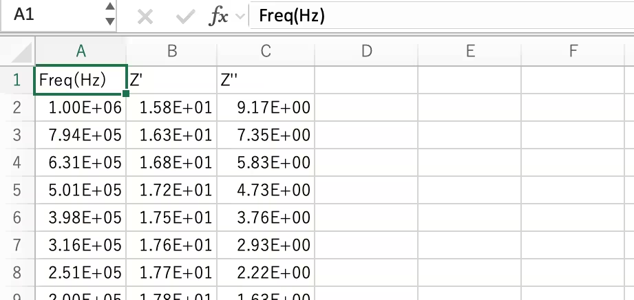
Place your data (Column A: Frequency, B: Z', C: Z'') starting from row 2 and run the ActiveSheetDRT_all macro.
Sub ActiveSheetDRT_all()
    ' 1. Data Prep (Magnitude/Phase calculation)
    Call CalculateMagAndPhase

    ' 2. Numerical Inversion (Main Computation)
    Call RunDRT

    ' 3. Parameter Optimization (L-Curve Method)
    Call FindOptimalLambda_Normalized

    ' 4. Model Reconstruction and Validation
    Call CalculateImpedanceFromOptimalDRT

    ' 5. Visualization
    Call CreateColeColeComparisonChart_Styled_A7
    Call CreateDRTSpectrumChart_Styled_G7
End Sub
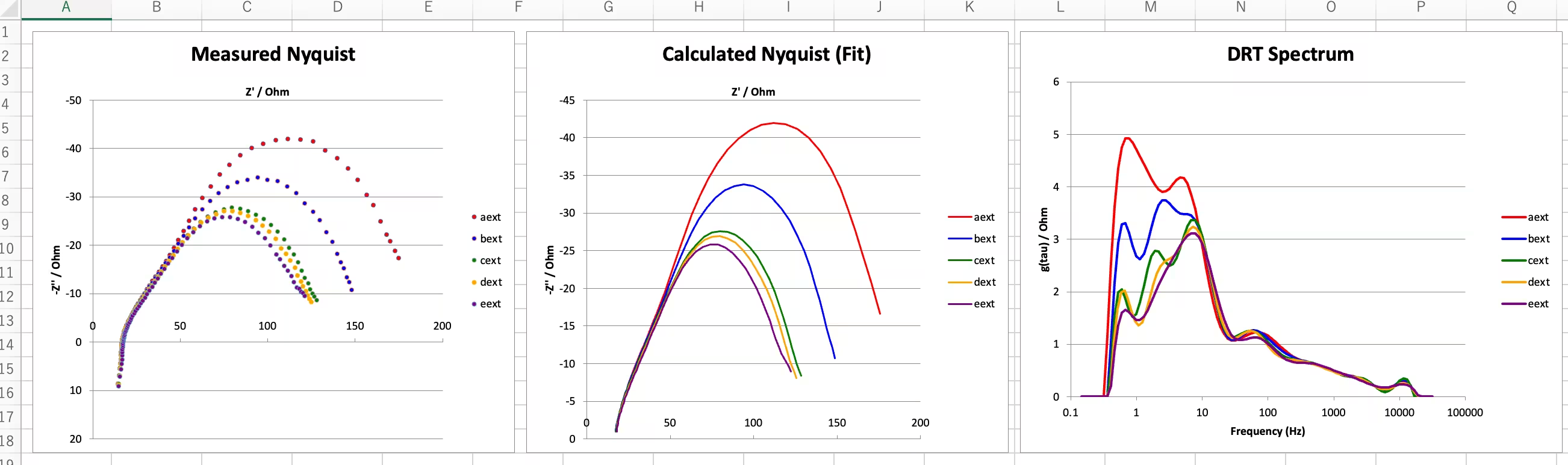
B. Option Feature (Batch Processing)
Designed for efficient processing of large datasets. By selecting multiple .z files via a dialog, the tool automates data extraction, continuous analysis, and comparison report generation.
To optimize efficiency, each dataset is assigned an individually optimized regularization parameter (λ). Please be aware that the final comparison graph may contain results calculated under different λ conditions.
.z files, but the loading logic can be easily modified for CSV or other formats.
4. Global Settings
Modify the constants at the top of the DRT_core module to control analysis behavior.
' 1. KK-Filter Threshold (%)
Public Const KK_THRESHOLD As Double = 3#

' 2. Lambda (λ) Scan Settings (10^0 to 10^-10)
Public Const LAMBDA_START_EXP As Double = 0#
Public Const LAMBDA_END_EXP As Double = 10#

' 3. DRT Spectrum Endpoint Trimming (Number of points to cut)
Public Const CUT_LOW_FREQ As Integer = 3
Public Const CUT_HIGH_FREQ As Integer = 0
5. Technical Deep Dive: Internal Processing
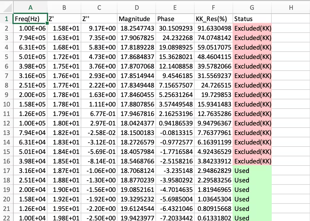
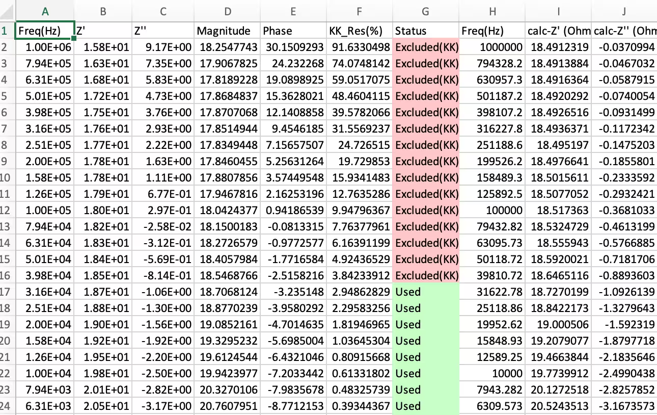
Step 1: Physical Consistency Verification (KK-Filter)
Verifies if EIS data is physically valid according to Kramers-Kronig relations. The tool checks the consistency of real and imaginary parts and excludes points where the deviation exceeds the KK_THRESHOLD (default 3%).
- Setting the Threshold: 3% to 5% is standard. Use 5% for noisy data and 1% for high-precision laboratory measurements.
- Why filter? Including points that violate KK relations due to drift or external noise can produce "ghost peaks" in the DRT spectrum.
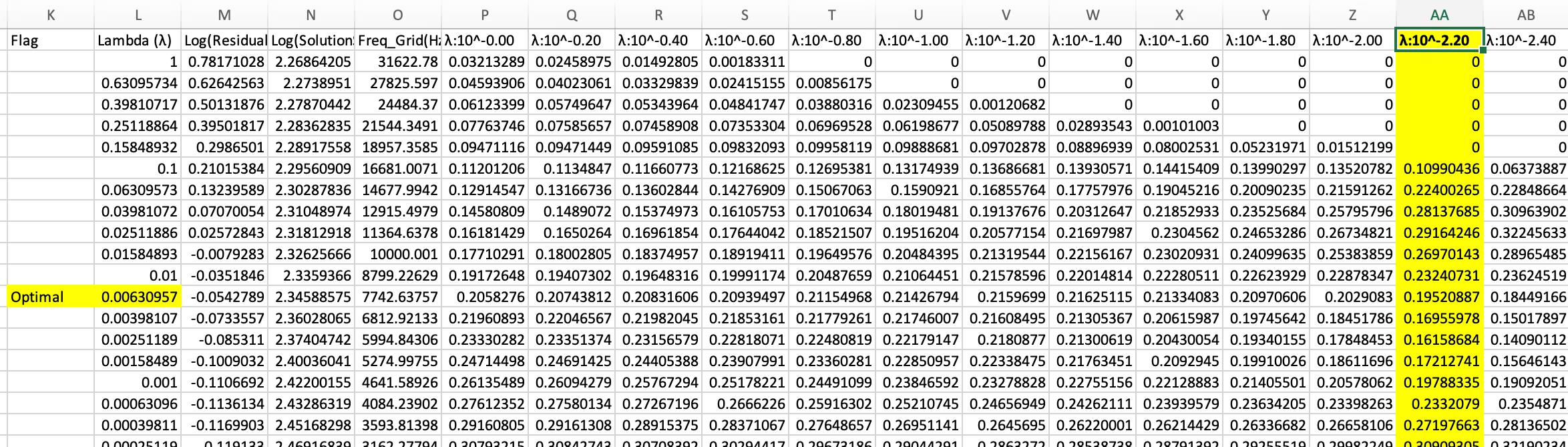
Step 2 & 3: Tikhonov Regularization and L-Curve Method
DRT calculation is an "ill-posed problem" where small noise can cause massive oscillations in the solution. We implement Tikhonov Regularization, adding a penalty term to ensure smoothness.
Auto-Optimization in VBA
Selecting the regularization strength "λ (lambda)" is critical for accurate results.
- λ Scan & Computation Time: The tool scans from
LAMBDA_START_EXPtoLAMBDA_END_EXP. Expanding this range improves the chance of finding the absolute optimum but increases calculation time due to the heavy matrix operations performed at each step. - L-Curve Evaluation: Residuals and Penalty are calculated for each λ. The "elbow point" (point of maximum curvature) on the L-curve is automatically selected as the most balanced λ.
Step 4: Reconstruction and Validation
The tool back-calculates impedance from the derived DRT to compare with raw data.
Frequency Endpoint Trimming
Mathematical artifacts often appear as sharp spikes at frequency boundaries. These can be removed by adjusting:
- Low-freq trim: Adjust
CUT_LOW_FREQ(e.g., 3 cuts the last 3 low-frequency points). - High-freq trim: Adjust
CUT_HIGH_FREQfor the high-frequency end.
6. References
- T. Reshetenko and A. Kulikovsky, "Understanding the distribution of relaxation times of a low–Pt PEM fuel cell," Electrochimica Acta, 391, 138954 (2021).
- C. Plank et al., "A review on the distribution of relaxation times analysis: A powerful tool for process identification of electrochemical systems," Journal of Power Sources, 594, 233845 (2024).
- Hirofumi Sumi, "Analysis of Electrochemical Impedance by Distribution of Relaxation Times (DRT) Method and Its Application," Denkikagaku, 90 (3), 279-286 (2022).
- Hirofumi Sumi's HomePage
- Z. Wang et al., "DRTtools: Freely Accessible Distribution of Relaxation Times Analysis for Electrochemical Impedance Spectroscopy," ACS Electrochemistry, 1 (12), 2680–2689 (2025).
- pyDRTtools (GitHub) - Ciucci's Lab.
7. License
This project is released under the MIT License. You are free to use, modify, and distribute it, provided the copyright notice is maintained.
EIS-DRT-Excel-Analyzer (日本語)
〜 企業のITセキュリティ制約を打破し、全てのエンジニアに高度なDRT解析を 〜
1. イントロダクション:本プロジェクトの「想い」
緩和時間分布(DRT)解析は、電気化学インピーダンス(EIS)データから物理現象を鮮やかに分離できる強力なツールです。現在、オンライン上でデータをアップロードして解析を行うクラウドサービスも存在しますが、機密情報を扱う多くのエンジニアにとって、外部サーバーへのデータアップロードは情報セキュリティ上の大きな障壁となっています。
本プロジェクトは、「ローカル環境のExcelだけで、専門ソフト並みの解析を完結させる」ことを目的としています。VBAコードとして提供されるため、IT部門による厳しいソフトウェアインストール制限を回避しつつ、機密データを一切外に出すことなく、あなたのデスクトップ上で安全に高度なDRT解析を行うことができます。
2. 使用方法 (Usage)
GitHub リポジトリ: @ykusachi/Excel_DRT
上記リンクより、VBAソースコードのコピーやテンプレートファイルのダウンロードが可能です。
モジュールの構成
DRT_core.bas:DRTのコアアルゴリズム。単一のインピーダンスデータから分布関数を導出します。Z_summary.bas:複数ファイルの一括解析用拡張機能。
Excelへの導入手順 (Windows / Mac 共通)
以下の手順で、OSを問わずVBAモジュールを導入できます。
- 解析を行いたいExcelファイルを開き、Visual Basic Editor (VBE) を起動します。
- Windows:
Alt + F11 - Mac:
Option + F11(または「ツール」メニュー > 「マクロ」 > 「Visual Basic Editor」)
- Windows:
- ファイルのインポート: VBEのメニューから「ファイル」>「ファイルのインポート...」を選択します。
- ダウンロードした
.basファイルを選択して読み込みます。 - 実行: Excel画面に戻り、「開発」タブ(または
Alt/Option + F8)からマクロを呼び出してください。
3. 解析機能の詳細
A. 解析コア機能(単体解析)
シート上の2行目以降にデータを配置(A列:周波数, B列:Z', C列:Z'')し、ActiveSheetDRT_all マクロを実行します。
Sub ActiveSheetDRT_all()
    ' 1. データ準備(絶対値・位相算出)
    Call CalculateMagAndPhase

    ' 2. 数値反転(メイン計算)
    Call RunDRT

    ' 3. パラメータ最適化(L-Curve法)
    Call FindOptimalLambda_Normalized

    ' 4. モデル再構成と検証
    Call CalculateImpedanceFromOptimalDRT

    ' 5. 可視化グラフ作成
    Call CreateColeColeComparisonChart_Styled_A7
    Call CreateDRTSpectrumChart_Styled_G7
End Sub
B. オプション機能(複数ファイル一括処理)
大量の実験データを効率的に処理するために設計されています。ダイアログから複数の .z ファイルを選択するだけで、データの抽出から連続解析、比較レポートの作成までを自動で行います。
本機能では、計算効率化のため各データに対して個別に最適化された正則化パラメータ(λ)が自動選定されます。比較グラフには、λが異なる条件での解析結果が混在する可能性があることに留意してください。
.z 形式対応ですが、読み込みロジックを修正すればCSV等あらゆるフォーマットに対応可能です。
4. 解析パラメータの詳細設定 (Global Settings)
モジュール上部の定数を変更することで、解析の挙動をコントロールできます。
' 1. KK-Filter Threshold (%)
Public Const KK_THRESHOLD As Double = 3#

' 2. Lambda (λ) Scan Settings (10^0 ~ 10^-10)
Public Const LAMBDA_START_EXP As Double = 0#
Public Const LAMBDA_END_EXP As Double = 10#

' 3. DRT Spectrum Endpoint Trimming (カットするデータ点数)
Public Const CUT_LOW_FREQ As Integer = 3
Public Const CUT_HIGH_FREQ As Integer = 0
5. 技術解説:解析プロセスの内部処理
Step 1: 物理的整合性の検証 (KK-Filter)
EISデータが物理的に妥当(Kramers-Kronig関係を満足)か検証します。本ツールでは、各周波数点での実部・虚部の整合性をチェックし、偏差がグローバルパラメータ KK_THRESHOLD(デフォルト 3%)を超える点を除外します。
- 閾値の決め方: 通常は3%〜5%程度が適当です。ノイズの多い測定データでは少し緩め(5%)に設定し、高精度な解析を求める場合は厳しめ(1%)に設定します。
- 除去のメリット: 経時変化や外部ノイズによりKK関係が崩れた点を含めて解析すると、DRTチャート上に物理的な意味のない「ゴーストピーク」が現れる原因となります。
Step 2 & 3: Tikhonov正則化とL-Curve法
DRT算出は「不良設定問題」であり、測定ノイズが解を激しく振動させます。本ツールではTikhonov正則化を導入し、解の滑らかさを保つペナルティ項を設けています。
VBAでの自動最適化
正則化の強度を決める「λ(ラムダ)」の選定は解析の肝となります。
- λの設定と計算時間:
LAMBDA_START_EXPからLAMBDA_END_EXPの範囲をスキャンします。スキャン範囲を広げるほど最適な点を見落としにくくなりますが、1点ごとに大規模な行列演算を行うため、計算時間が長くなります。 - L-Curveの評価: 各λにおける再現性(Residual)と解の滑らかさ(Penalty)を算出し、そのトレードオフ曲線において曲率が最大となる「エルボー点」を、客観的に最も妥当なλとして自動採用します。
Step 4: インピーダンス再構成と検証
得られたDRTからインピーダンスを逆計算し、実測値と比較します。
周波数端のポイントカット
測定範囲の両端では数学的制約によりDRT強度が跳ね上がるアーティファクトが生じやすいため、グローバルパラメータで調整が可能です。
- 低周波端:
CUT_LOW_FREQの値を調整(例:3なら低周波側3点をカット)。 - 高周波端:
CUT_HIGH_FREQの値を調整。
6. 参考文献 (References)
- T. Reshetenko and A. Kulikovsky, "Understanding the distribution of relaxation times of a low–Pt PEM fuel cell," Electrochimica Acta, 391, 138954 (2021).
- C. Plank et al., "A review on the distribution of relaxation times analysis: A powerful tool for process identification of electrochemical systems," Journal of Power Sources, 594, 233845 (2024).
- Hirofumi Sumi, "緩和時間分布(DRT)法による電気化学インピーダンス解析とその応用," Denkikagaku, 90 (3), 279-286 (2022).
- Hirofumi Sumi's HomePage
- Z. Wang et al., "DRTtools: Freely Accessible Distribution of Relaxation Times Analysis for Electrochemical Impedance Spectroscopy," ACS Electrochemistry, 1 (12), 2680–2689 (2025).
- pyDRTtools (GitHub) - Ciucci's Lab.
Cite This Tool (BibTeX)
@misc{kusachi2025exceldrt,
  author = {Yuki Kusachi},
  title = {EIS-DRT-Excel-Analyzer (Electrochemical Impedance DRT Analysis in Microsoft Excel)},
  year = {2025},
  url = {https://www.edandc.com/Excel-DRT/},
  note = {YK Energy Device \& Consulting}
}
7. ライセンス (License)
本プロジェクトは MITライセンス の下で公開されています。商用利用・改変・再配布が可能ですが、著作権表示を保持してください。