Can Ultra-Fast Pulse and High-Frequency EIS Diagnostics Decouple Battery Degradation Modes? Insights from Physics Simulations & Machine Learning
Executive Summary: Core Findings of This Study
In electric vehicles (EVs) and stationary energy storage systems, can individual degradation modes inside the battery—such as positive/negative active material loss, lithium inventory loss, SEI layer thickening, pore clogging, and reaction kinetics decay—be decoupled in just a few seconds upon full charge completion?
Using PyBaMM's Doyle-Fuller-Newman (DFN/P2D) electrochemical physics model and deep learning across four experimental phases (Phase 1 to Phase 4), we uncovered both decisive breakthroughs and unavoidable physical limits:
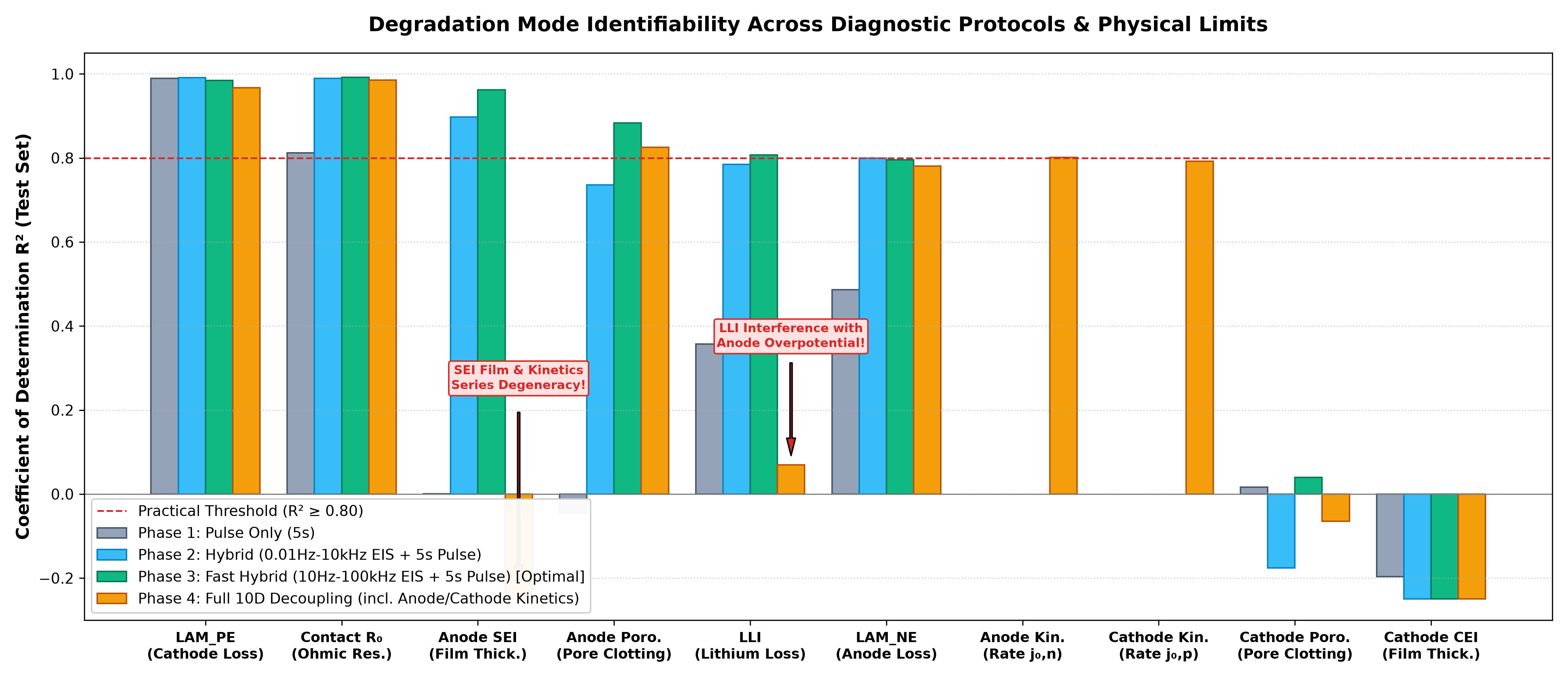
- Limits of Pulse Only (5s): Because all overpotential components are serially summed in the terminal voltage, only cathode active material loss (LAM_PE, $R^2=0.990$) with its steep equilibrium potential slope and pure contact resistance ($R_0, R^2=0.812$) can be identified. Anode SEI thickness, porosity loss, and LLI yield $R^2 \approx 0$ and cannot be isolated.
- Breakthrough of Fast EIS (10 Hz–100 kHz, 0.5s) + Pulse (5s): In a combined diagnostic protocol taking only ~5.5 seconds, time-constant separation isolates the ohmic intercept and interface film impedance. Anode SEI thickness ($R^2=0.962$, MAE 1.14 nm), anode porosity reduction ($R^2=0.884$), lithium inventory loss (LLI, $R^2=0.807$), and anode active material loss (LAM_NE, $R^2=0.795$) are simultaneously decoupled with high accuracy under fixed kinetics.
- The "Series Degeneracy Barrier" under Variable Kinetics: When degradation-induced degradation of exchange-current density ($i_0$) is introduced as an unknown parameter (10-dimensional space), anode SEI film resistance $R_{\text{sei}}$ and charge transfer resistance $R_{\text{ct}}$ form an exact series combination. They mutually cancel, causing the individual identifiability of SEI thickness and LLI to collapse—a fundamental mathematical limit demonstrated empirically.
Degradation Mode Identifiability ($R^2$) Across Diagnostic Protocols and Physical Limits
Comparison of coefficient of determination ($R^2$) on an unseen test dataset (50 cells with randomized manufacturing prior variations). Phase 3 demonstrates dramatic improvements across interfacial and transport parameters, while Phase 4 demonstrates specific degradation in SEI thickness and LLI due to series resistance degeneracy.
1. Background & Motivation: Why Do We Need Sub-Second / Multi-Second Screening?
To truly understand a lithium-ion battery's State of Health (SOH), observing overall remaining discharge capacity alone is insufficient. Multiple distinct physicochemical mechanisms drive capacity and power fade:
- LLI (Loss of Lithium Inventory): Consumption of cyclable lithium via continuous SEI film growth and metallic lithium plating on the negative electrode.
- LAM (Loss of Active Material): Delamination or particle fracture caused by lattice strain during intercalation, isolating active particles from conductive pathways (positive electrode $\text{LAM}_{\text{PE}}$, negative electrode $\text{LAM}_{\text{NE}}$).
- Pore Clogging (Porosity Reduction): Deposition of decomposition products within electrode pores, drastically increasing electrolyte liquid-phase diffusion resistance.
- Kinetics Degradation: Interfacial passivation and surface phase transformations reducing the exchange-current density $i_0$ for charge transfer.
Decoupling these parameters enables adaptive BMS controls—such as throttling peak charging current if anode pores are severely clogged, or lowering the top-of-charge voltage limit if cathode material loss has accelerated.
The Real-World Dilemma: Full-Discharge Tests and Low-Frequency EIS Are Impractical in the Field
In laboratory settings, low-rate C/20 discharge tests for incremental capacity / differential voltage analysis (ICA/DVA) or low-frequency EIS down to 0.01 Hz can cleanly decouple these degradation modes.
However, a C/20 discharge requires over 20 hours, and a 0.01 Hz EIS point requires 100 seconds for a single sinusoidal cycle (multiple minutes for a spectrum).
To satisfy the operational requirement of "safely completing an automated health check in just a few seconds right after an overnight AC charge completes," extracting internal state variables from short current pulses and high-frequency spectroscopy is critical.
2. Diagnostic Protocol Design & Full-Charge (100% SOC) Operating Condition
[Key Premise] Diagnostic Condition: Fully Charged State (100% SOC, 4.20 V)
All pulse transient responses and high-frequency EIS sweeps in this study were simulated at "Initial 100% SOC (4.20 V fully charged state)." This condition targets automated screening executed immediately upon completing an AC overnight or depot charge, rather than low-SOC arrival at a public fast charger.
[Critical Caveat] Protocol is an Illustrative Baseline & Practical Discrepancy from Post-Charge Temperature Rise
1. Setting is an Illustrative Example: The protocol parameters demonstrated here (100% SOC, 5C pulse, high-frequency EIS band) serve as a representative baseline designed to investigate the mathematical limits of degradation decoupling under controlled conditions.
2. Post-Charge Cell Heating Causes Practical Discrepancy: In real-world battery operations, continuous charging up to 100% SOC inevitably produces substantial internal Joule heating ($I^2 R$) and reversible entropic heat ($I T \frac{\partial U}{\partial T}$), causing cell temperature to rise above ambient by several degrees or more upon charge completion. Because this simulation assumes an ideal isothermal condition ($25^\circ\text{C}$ constant) without coupling a thermal model, raw measurements taken directly on physical cells immediately after full charge will naturally deviate from these simulation results. Interfacial kinetics ($i_0$), solid/liquid diffusion ($D_s, D_e$), and electrolyte conductivity ($\kappa$) follow strong Arrhenius temperature dependence ($\propto \exp(-E_a/RT)$). Deploying this methodology in practice strictly requires thermistor monitoring and temperature compensation maps or training across multi-temperature datasets.
We targeted commercial high-energy LG M50 21700 cylindrical cells (5.0 Ah, NMC811 / Si-graphite composite anode) using PyBaMM's Doyle-Fuller-Newman (DFN) electrochemical model.
Proposed Diagnostic Protocol (Total 6.0 Seconds)
- Step 1: Fast EIS Sweep (0.5s): 25 logarithmically spaced frequencies from $100\text{ kHz}$ down to $10\text{ Hz}$ at 0.2C (1.0 A) amplitude. Scans the pure ohmic intercept and the high-frequency SEI film / double-layer arc.
- Step 2: High-Rate Charge Pulse (2.5s): +5.0C (25.0 A). Excites strong field-driven overpotential buildup and active material open-circuit voltage response.
- Step 3: Diagnostic Rest (0.5s): 0 A. Measures the open-circuit relaxation trajectory and double-layer discharge dynamics after instantaneous IR drop collapse.
- Step 4: Restorative Discharge Pulse (2.5s): -3.0C (-15.0 A). Forms a Bidirectional Pulse Response (BPR) to cancel accumulated charge, ensuring negligible net SOC shift ($\\Delta \text{SOC} \approx 0.1\%$).
Simulation Realism: Unobserved Manufacturing Prior Variations (Noise)
To prevent artificial overfitting to an idealized cell, all samples were co-perturbed with 6-dimensional random manufacturing tolerances:
3. Electrochemical Physics Model, Dataset Generation, Neural Architecture, & Validation
This section provides full technical details of the simulation model, sampling protocol, deep learning network architecture, and evaluation metrics.
(1) PyBaMM Electrochemical Physics Model Specification
Simulations were executed using PyBaMM (Python Battery Mathematical Modelling, v26.10):
- Governing Physics: Standard Doyle-Fuller-Newman (DFN / P2D) model coupling Fickian solid-state diffusion within spherical active particles, concentrated solution electrolyte transport (Nernst-Planck), and nonlinear Butler-Volmer interface charge transfer across the cell thickness.
- Cell Parameterization: Parameter sets
OKane2022andChen2020for commercial LG M50 21700 cells (5.0 Ah). Cathode: NMC811 ($75.6\ \mu\text{m}$); Anode: Si-graphite composite ($85.2\ \mu\text{m}$); Electrolyte: $1.0\text{ M LiPF}_6$ (EC:EMC 3:7 wt%). - Submodel Options:
- Film Growth & Pore Clogging: Negative SEI growth modelled via
pybamm.sei.ReactionDriven, dynamically tracking pore volume reduction (Porosity Reduction) coupled to film thickening. - Double-Layer Capacitance: Interfacial double-layer capacitance $C_{\text{dl}}$ included to capture capacitive current bypass under fast transient transitions.
- Numerical Solvers: Time-domain pulse solved with
IDAKLUSolver(SUNDIALS/IDA stiff DAE solver); impedance spectra solved withpybamm.EISSimulation. - Thermal Dynamics:
isothermal($T = 25^\circ\text{C}$). Thermal energy conservation was uncoupled to isolate baseline electrical identifiability without thermal cross-talk.
- Film Growth & Pore Clogging: Negative SEI growth modelled via
(2) Latin Hypercube Sampling & Dataset Generation
To uniformly cover the multi-dimensional parameter space, Latin Hypercube Sampling (LHS / Sobol sequences, scipy.stats.qmc) was utilized to generate 500 samples per phase.
- Degradation Target Parameters:
- Positive active material loss (LAM_PE): 0.0% to 20.0%
- Negative active material loss (LAM_NE): 0.0% to 20.0%
- Loss of lithium inventory (LLI): 0.0% to 20.0%
- Negative SEI thickness $\delta_{\text{sei}}$: 5.0 nm to 30.0 nm
- Positive CEI thickness $\delta_{\text{cei}}$: 2.0 nm to 15.0 nm
- Negative porosity reduction $\Delta \varepsilon_{\text{ne}}$: 0.0% to 35.0%
- Positive porosity reduction $\Delta \varepsilon_{\text{pe}}$: 0.0% to 35.0%
- Contact ohmic resistance $R_0$: 0.0 to 10.0 $\text{m}\Omega$
- (Phase 4) Negative exchange-current density hindrance $\Delta j_{0,\text{ne}}$: 0.0% to 80.0%
- (Phase 4) Positive exchange-current density hindrance $\Delta j_{0,\text{pe}}$: 0.0% to 80.0%
- Input Feature Vectors:
- Frequency Domain (EIS): Real $\mathrm{Re}(Z)$ and imaginary $-\mathrm{Im}(Z)$ impedance across 25 frequencies (50 dimensions).
- Time Domain (Pulse): Voltage $V(t)$, current $I(t)$, and time-derivative $\mathrm{d}V/\mathrm{d}t$ across 501 points ($2 \times 501$ dimensions).
- Physics Scalar Metrics: 12 summary features (instantaneous IR drop, relaxation slopes, high-frequency intercept).
(3) Deep Learning Architecture: Dual-Domain Hybrid Estimator
To fuse heterogeneous time-series and spectral inputs, a custom multi-branch deep neural network was constructed in PyTorch:
- Branch 1 (Pulse Waveform): 1D-ResNet (3 residual stages, SiLU activation, BatchNorm1D, AdaptiveAvgPool1D) compressing transient trajectories into a 64-dimensional latent embedding.
- Branch 2 (EIS Spectrum): 1D-CNN (3 convolutional layers, SiLU, AdaptiveAvgPool1D) extracting Nyquist semicircle curvature and apex frequencies into a 64-dimensional latent embedding.
- Branch 3 (Scalar Metrics): 2-layer MLP projecting 12 summary features into a 32-dimensional embedding.
- Feature Fusion Head: Concatenated representation ($64 + 64 + 32 = 160$ dimensions) passed through dense layers ($160 \rightarrow 128 \rightarrow 64$, Dropout 0.1) for simultaneous multi-task regression output.
- Training Configuration: Optimized using Huber Loss (Smooth L1 Loss) with AdamW (initial learning rate $1 \times 10^{-3}$, Cosine Annealing, Weight Decay $1 \times 10^{-4}$, Early Stopping).
(4) Statistical Validation Protocol
- Dataset Split: 500 samples partitioned strictly into Train (400, 80%), Validation (50, 10%), and Test (50, 10%) sets. The test set was held out exclusively for final model benchmarking.
- Coefficient of Determination ($R^2$): $$R^2 = 1 - \frac{\sum_{i=1}^N (y_i - \hat{y}_i)^2}{\sum_{i=1}^N (y_i - \bar{y})^2}$$ Evaluates variance explained relative to ground truth ($R^2 \ge 0.80$ defined as practical decoupling threshold; $R^2 \le 0$ denotes failure).
- Mean Absolute Error (MAE): Evaluated directly in physical units (%, nm, $\text{m}\Omega$).
- Parity & Residual Testing: Inspected visually via parity scatter plots ($y = x$) to ensure absence of systemic bias.
4. Trajectory Across the Four Experimental Phases
Phase 1: Pulse Only (5s)
Series Overpotential BarrierInputs only 5-second pulse waveforms. High cathode OCV slope enables LAM_PE decoupling ($R^2=0.990$), but SEI thickness, porosity loss, and LLI are masked by series overpotentials ($R^2 \approx 0$).
Phase 2: Low-Freq EIS + Pulse
0.01 Hz BreakthroughCombines wideband EIS (0.01 Hz–10 kHz). Accuracy dramatically rises for SEI thickness ($R^2=0.898$), LLI ($R^2=0.784$), and porosity ($R^2=0.736$). However, 0.01 Hz requires 100s per cycle.
Phase 3: Fast EIS (10Hz–100kHz) + Pulse
Optimal Real-World Solution ★Reduces EIS duration to 0.5s while expanding to 100 kHz. Pure ohmic intercept is exposed, delivering peak accuracy: SEI thickness ($R^2=0.962$, MAE 1.14 nm), porosity ($R^2=0.884$), and LLI ($R^2=0.807$).
Phase 4: Variable Kinetics (10 Targets)
Empirical Proof of Series DegeneracyAdds exchange-current densities as free targets. Reaction kinetics themselves are decoupled ($R^2 \approx 0.80$), but series combination of $R_{\text{sei}}$ and $R_{\text{ct}}$ collapses SEI thickness identifiability.
5. Quantitative Benchmark & Accuracy Comparison Table
| Degradation Parameter | Unit | Phase 1 (5s Pulse) | Phase 2 (Low-Freq EIS+Pulse) | Phase 3 (Fast EIS+Pulse) ★ | Phase 4 (10D incl. Kinetics) | Verdict | Physical Mechanism & Origin |
|---|---|---|---|---|---|---|---|
| Cathode Active Material Loss (LAM_PE) | % | $R^2 = 0.9899$ MAE: 0.72% |
$R^2 = 0.9911$ MAE: 0.65% |
$R^2 = 0.9844$ MAE: 0.85% |
$R^2 = 0.9668$ MAE: 1.10% |
Decoupled | Steep equilibrium potential slope (dOCV/dy) of NMC811 at 100% SOC dominates pulse transient response. |
| Contact / Tab Ohmic Resistance ($R_0$) | $ ext{m}\Omega$ | $R^2 = 0.8124$ MAE: 0.38 $ ext{m}\Omega$ |
$R^2 = 0.9898$ MAE: 0.08 $ ext{m}\Omega$ |
$R^2 = 0.9918$ MAE: 0.07 $ ext{m}\Omega$ |
$R^2 = 0.9851$ MAE: 0.09 $ ext{m}\Omega$ |
Decoupled | 100 kHz real-axis intercept cleanly separates bulk electrolyte and electronic resistance from capacitive loops. |
| Negative SEI Layer Thickness | nm | $R^2 = 0.0007$ MAE: 7.73 nm |
$R^2 = 0.8979$ MAE: 1.95 nm |
$R^2 = 0.9620$ MAE: 1.14 nm |
$R^2 = -0.8998$ MAE: 9.38 nm (Degenerate) |
Conditional | Fully decoupled via high-frequency arc under fixed kinetics; degenerates when exchange current varies. |
| Negative Porosity Reduction (Poro_NE) | % | $R^2 = -0.0441$ MAE: 4.88% |
$R^2 = 0.7358$ MAE: 2.14% |
$R^2 = 0.8838$ MAE: 1.48% |
$R^2 = 0.8254$ MAE: 1.63% |
Decoupled | 5C pulse drives pronounced liquid-phase pore overpotential, matching mid-frequency electrolyte impedance. |
| Loss of Lithium Inventory (LLI) | % | $R^2 = 0.3567$ MAE: 2.39% |
$R^2 = 0.7844$ MAE: 1.18% |
$R^2 = 0.8074$ MAE: 1.10% |
$R^2 = 0.0699$ MAE: 2.76% (Degenerate) |
Conditional | Drives local electrode stoichiometry shifts; suffers cross-interference with anode overpotential in Phase 4. |
| Anode Active Material Loss (LAM_NE) | % | $R^2 = 0.4865$ MAE: 3.51% |
$R^2 = 0.7998$ MAE: 1.76% |
$R^2 = 0.7953$ MAE: 1.83% |
$R^2 = 0.7806$ MAE: 1.87% |
Decoupled | Graphite stage-transition boundaries reflected in the tail of relaxation trajectories after pulse excitation. |
| Anode Exchange Current Density (Kin_NE) | % | — | — | — | $R^2 = 0.8014$ MAE: 4.88% |
Identifiable | Butler-Volmer non-linear charge transfer resistance directly drives initial pulse overpotential rise. |
| Cathode Exchange Current Density (Kin_PE) | % | — | — | — | $R^2 = 0.7922$ MAE: 4.67% |
Identifiable | Cathode charge transfer time-constant surfaces in the hundred-Hz to kHz frequency band of the EIS spectrum. |
| Positive Porosity Reduction (Poro_PE) | % | $R^2 = 0.0168$ | $R^2 = -0.1757$ | $R^2 = 0.0399$ | $R^2 = -0.0650$ | Invisible | Cathode is thin ($75.6\ \mu\text{m}$); liquid-phase ohmic drop accounts for <1% of overpotential. |
| Positive CEI Layer Thickness | nm | $R^2 = -0.1965$ | $R^2 = -0.4015$ | $R^2 = -0.3407$ | $R^2 = -0.5056$ | Invisible | CEI film is ultra-thin (1.5–3 nm) and ionically conductive; terminal overpotential contribution is <0.1 mV. |
6. In-Depth Parameter Decoupling Analysis
(1) Benchmark Parity Verification (Phase 3 Optimal Protocol)
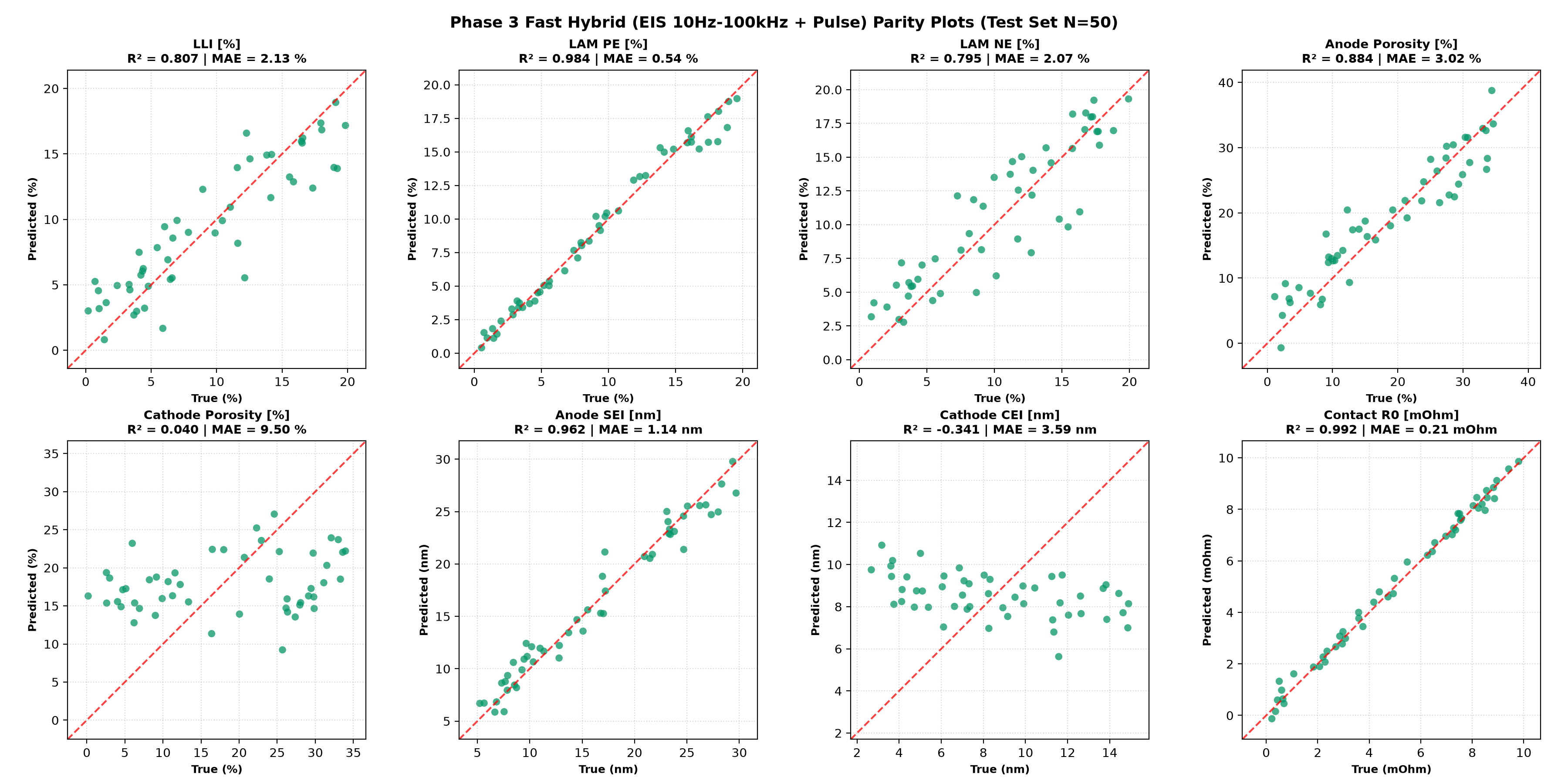
Predicted versus ground-truth scatter plots across the unseen test set for Phase 3. Points clustered along the red dashed diagonal ($y=x$) indicate high decoupling fidelity:
Phase 3: Parity Scatter Plots Across 8 Degradation Targets
LAM_PE ($R^2=0.984$), Contact R0 ($R^2=0.992$), Anode SEI ($R^2=0.962$), Anode Porosity ($R^2=0.884$), LLI ($R^2=0.807$), and LAM_NE ($R^2=0.795$) exhibit linear decoupling. Cathode CEI and porosity are completely flat (undetectable).
(2) Why Positive CEI and Cathode Porosity are Fundamentally "Invisible"
Across all four phases, cei_thickness_p and delta_poro_pe persistently yielded negative $R^2$ values. This is governed by strict electrochemical physics:
- CEI Film Resistance is Negligible: Compared to negative SEI (growing from 5 nm to 30 nm), cathode CEI remains exceedingly thin (1.5 to 3 nm) and exhibits higher ionic conductivity. Resulting overpotential drop across the CEI is below $0.1\text{ mV}$, completely buried under manufacturing tolerances.
- Cathode Liquid Diffusion is Not Limiting: In the LG M50 design, the cathode is relatively thin ($75.6\ \mu\text{m}$) compared to the anode ($85.2\ \mu\text{m}$) and has lower tortuosity. Liquid-phase electrolyte depletion is strictly anode-limited, meaning terminal voltage reflects anode pore clogging almost exclusively.
(3) Observation Point Condition: Why 100% SOC Enables Exceptional LAM_PE Decoupling
One of the most striking results is the near-perfect identification of LAM_PE ($R^2 \approx 0.99$) even in Phase 1 ($R^2 = 0.9899$). This success is fundamentally tied to the fully charged operating condition (SOC 100%):
Electrochemical Origin of High Cathode Identifiability at 100% SOC:
The open-circuit potential curve $U_{\text{pe}}(y)$ of NMC811 exhibits an extremely steep slope ($\\mathrm{d}U_{\text{pe}}/\\mathrm{d}y$) near the upper cutoff voltage ($> 4.1\text{ V vs Li/Li}^+$):
- Cathode OCV Amplification: When active cathode material is lost ($\text{LAM}_{\text{PE}}$), the remaining particles experience larger stoichiometric lithium shifts $\\Delta y$. Because $\\mathrm{d}U_{\text{pe}}/\\mathrm{d}y$ is nearly vertical at 100% SOC, even a 2.5-second pulse produces a prominent equilibrium voltage shift ($\\Delta V_{\text{ocv}} \approx \frac{\\mathrm{d}U_{\text{pe}}}{\\mathrm{d}y} \\Delta y$), giving the neural network an unmistakable signal.
- Anode Potential Flatness: In contrast, the graphite anode at 100% SOC rests in the Stage 1 intercalation plateau ($\\approx 0.08\text{ V vs Li/Li}^+$), where its potential slope is virtually flat ($\\mathrm{d}U_{\text{ne}}/\\mathrm{d}x \approx 0$). Consequently, pulse voltage changes at 100% SOC reflect cathode dynamics in almost pure isolation.
7. Electrochemical Origin of Degradation Decoupling & Series Degeneracy
Mathematical Proof: Why Did SEI Thickness and LLI Collapse in Phase 4?
In Phase 3, SEI thickness was predicted with $R^2 = 0.9620$. In Phase 4, when exchange-current density was treated as a variable degradation parameter, $R^2$ plummeted to $-0.8998$. The mathematical origin lies in the interface overpotential equation:
Series Overpotential Summation:
Under an interfacial current density $j$, total interfacial overpotential $\eta_{\text{interface}}$ is the series addition of film ohmic drop and charge-transfer overpotential $\eta_{\text{ct}}$:
$$\eta_{\text{interface}} = j \cdot R_{\text{sei}} + \eta_{\text{ct}} \approx j \cdot \left( \frac{\delta_{\text{sei}}}{\kappa_{\text{sei}}} + \frac{R T}{\alpha F \cdot i_{0,\text{NE}}} \right)$$
where $\delta_{\text{sei}}$ is film thickness, $\kappa_{\text{sei}}$ is film conductivity, and $i_{0,\text{NE}}$ is exchange-current density.
- Phase 3 (Fixed Kinetics): The second term ($\frac{RT}{\alpha F i_0}$) is invariant. Any observed shift in interface resistance maps one-to-one to $\delta_{\text{sei}}$, enabling precise neural estimation.
- Phase 4 (Variable Kinetics): Thickening the SEI film (increasing $\delta_{\text{sei}}$) and degrading kinetics (decreasing $i_0$) generate identical ohmic-like series resistance increments at the cell terminals. From external measurements alone at a single operating point, disentangling the two terms becomes mathematically ill-posed (solution degeneracy).
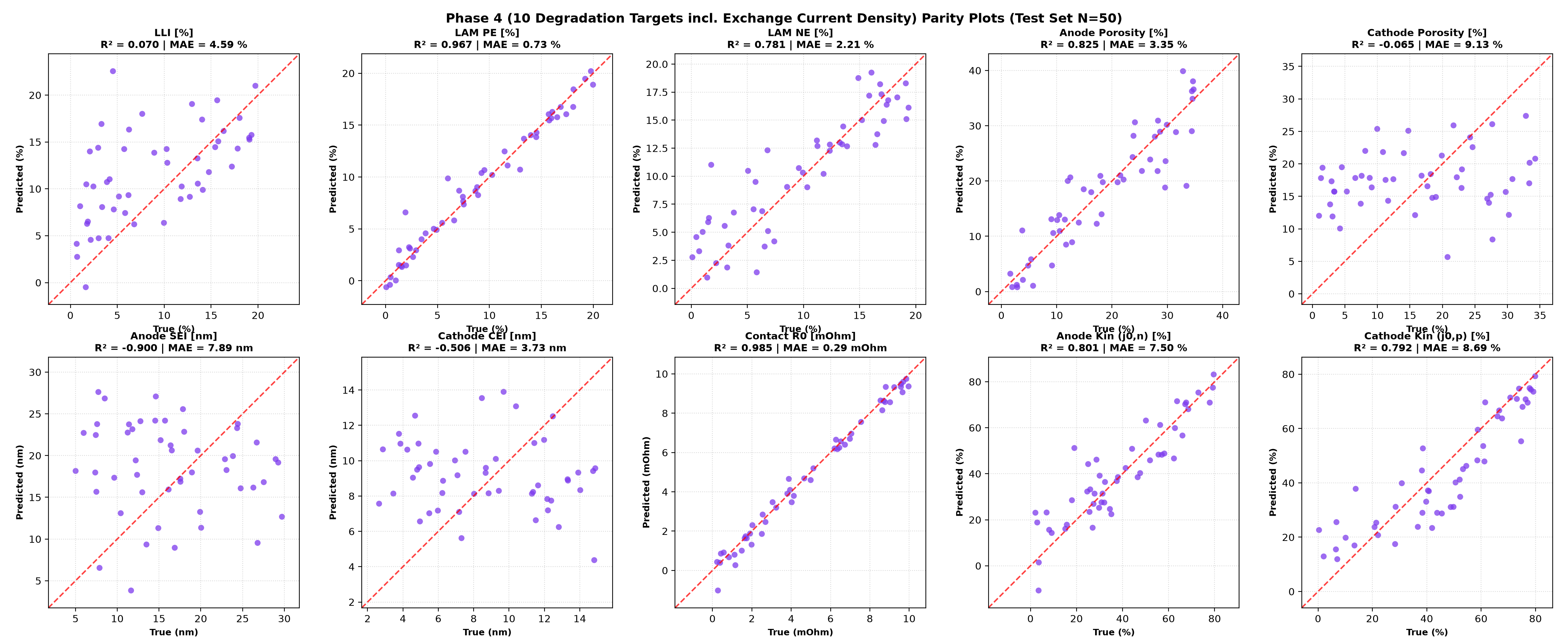
Phase 4: Parity Scatter Plots Across 10 Degradation Targets (Proof of Degeneracy)
While exchange current rates (Anode Kin, Cathode Kin) achieve $R^2 \approx 0.80$, the top-row third plot (Anode SEI) exhibits severe horizontal dispersion due to mutual overpotential cancellation with reaction kinetics.
8. Real-World BMS & Infrastructure Implementation Scenario
Because this protocol requires an initial 100% SOC (fully charged state), it is ideally tailored for automated diagnostic screening upon completing an overnight AC charge (home/depot) or post-manufacturing end-of-line verification, rather than midway fast charging stops.
Post-Full-Charge Automated 6-Second Health Screening Sequence
- Full Charge Trigger (100% SOC): As the AC charger terminates at 4.20 V, the vehicle initiates the screening routine prior to contactor opening.
- 0.0s – 0.5s (High-Frequency EIS Sweep): On-board charger or motor inverter injects small-signal AC (1.0 A) from 100 kHz down to 10 Hz to isolate $R_0$ and high-frequency SEI impedance.
- 0.5s – 3.0s (High-Rate Pulse Test): 5C (25 A) pulse captures steep cathode OCV response for $\text{LAM}_{\text{PE}}$ and pore diffusion overpotentials for anode porosity reduction.
- 3.0s – 3.5s (Zero-Current Relaxation): Open-circuit voltage relaxation records double-layer discharge kinetics.
- 3.5s – 6.0s (Restorative Discharge): Brief 3C (15 A) discharge returns net cell charge to safe thresholds (preventing overcharge; net $\Delta \text{SOC} \approx 0.1\%$).
- 6.0s Completion (Adaptive BMS Feedback):
- If Anode Porosity is Clogged: BMS automatically throttles maximum allowable fast-charge current maps to prevent liquid-phase salt depletion and lithium plating.
- If Cathode Material Loss ($\text{LAM}_{\text{PE}}$) is Severe: Top-of-charge cutoff voltage is slightly derated (e.g., from 4.20 V to 4.15 V) to avoid excessive high-voltage structural degradation.
Prerequisite for Real-World Deployment: Post-Charge Thermal Dynamics & Temperature Compensation
As noted, this simulation assumes an ideal $25^\circ\text{C}$ isothermal environment as an illustrative baseline. In actual EVs, continuous charging to 100% SOC elevates cell temperature (typically $30^\circ\text{C}$–$45^\circ\text{C}$ depending on ambient conditions and charge C-rate).
- Mechanism of Thermal Discrepancy: Elevated temperature accelerates Butler-Volmer kinetics ($i_0$) and diffusion ($D_e, D_s$), compressing both activation and pore concentration overpotentials. Consequently, uncorrected raw post-charge data would lead the estimator to underestimate degradation (e.g., perceiving SEI thickness or porosity loss to be milder than reality).
- BMS Implementation Architecture: An operational BMS must capture the cell thermistor reading ($T_{\text{cell}}$) simultaneously with the 6-second pulse, applying Arrhenius scaling maps to normalize the measured overpotential $\eta(t)$ and impedance $Z(\omega)$ to $25^\circ\text{C}$ baseline equivalents prior to neural network inference.
9. Summary: What Can and Cannot Be Done in Ultra-Fast Diagnostics
What CAN Be Decoupled in Ultra-Fast Testing:
- Cathode Active Material Loss ($\text{LAM}_{\text{PE}}$) and Ohmic Resistance ($R_0$) at 100% SOC: The steep dU/dy slope of NMC811 enables $R^2 \ge 0.81$ with 5s pulse alone, and $R^2 \ge 0.98$ when paired with high-frequency EIS.
- Simultaneous 4-Mode Decoupling via Fast EIS (10 Hz–100 kHz) + Pulse: In ~5.5 seconds, SEI thickness ($R^2=0.962$), anode porosity loss ($R^2=0.884$), LLI ($R^2=0.807$), and anode material loss $\text{LAM}_{\text{NE}}$ ($R^2=0.795$) are decoupled simultaneously under unobserved manufacturing variations.
What CANNOT Be Decoupled (Fundamental Physical Limits):
- Cathode CEI Thickness and Cathode Porosity (Invisible): Thin CEI layers (1.5 nm) and small cathode diffusion overpotentials (<1% of cell overpotential) make them completely invisible at the cell terminals.
- Independent SEI Thickness and LLI Separation Under Variable Reaction Kinetics (Series Degeneracy): Film resistance $R_{\text{sei}}$ and charge transfer resistance $R_{\text{ct}}$ form an inseparable series combination; single-point terminal diagnostics cannot mathematically isolate them when kinetics are unconstrained.
- Direct Application to Non-Isothermal Real Cells Without Temperature Compensation: The current setting is an illustrative baseline example under isothermal $25^\circ\text{C}$. Because continuous charging causes internal heat generation, raw post-charge physical data will mismatch the model unless cell temperature is monitored and compensated via Arrhenius scaling or multi-temperature training.
10. References & Key Patents
- Newman P2D Benchmark Model: M. Doyle, T. F. Fuller, and J. Newman, "Modeling of Galvanostatic Charge and Discharge of the Lithium/Polymer/Insertion Cell," Journal of The Electrochemical Society, 140(6), 1526-1533, 1993. doi:10.1149/1.2221597
- LG M50 21700 Parameterization: C.-H. Chen et al., "Development of Experimental Techniques for Parameterization of Multi-Scale Lithium-Ion Battery Models," Journal of The Electrochemical Society, 167(8), 080534, 2020. doi:10.1149/1945-7111/ab9050
- PyBaMM Degradation Model: S. E. J. O'Kane et al., "Physical origin of the differential voltage minimum associated with lithium plating in Li-ion cells," Physical Chemistry Chemical Physics, 24(13), 7909-7922, 2022. doi:10.1039/D2CP00417H
- Machine Learning Degradation Review: Y. Zhang, Q. Tang, et al., "Identifying degradation modes of lithium-ion batteries via machine learning," Nature Communications, 11, 4477, 2020. doi:10.1038/s41467-020-18276-4
- Dynamic Impedance Screening Patents: US Patent Nos. 10,218,200 / 11,237,216.
If you found these physics-based simulation insights valuable, please consider supporting our continuous open-access publications!
Cite this Article (BibTeX)
@article{kusachi2026fastdiagnostics,
  author = {Yuki Kusachi},
  title = {Can Ultra-Fast Pulse and High-Frequency EIS Diagnostics Decouple Battery Degradation Modes? Insights from Physics Simulations & Machine Learning},
  journal = {YK Energy Device \& Consulting Technical Insights},
  year = {2026},
  url = {https://www.edandc.com/articles/FastPulse_EIS_Degradation_Decoupling.html}
}